Discounted Cash Flow (DCF) valuation is a method that estimates a company's intrinsic value by forecasting its future cash flows and discounting them to present value. For serious investors, building a DCF from the ground up improves conviction, highlights key value drivers, and exposes model risk.
This article teaches an advanced, repeatable process: projecting financials (revenue growth, margins, working capital, capex), converting to free cash flow, selecting a discount rate (WACC or alternatives), computing terminal value, and conducting sensitivity analysis. Expect practical examples, numeric walk-throughs, and implementation tips for spreadsheet models.
- DCF isolates intrinsic value by modeling Free Cash Flow to Firm (FCFF) and discounting at the appropriate rate (usually WACC).
- Accurate projections hinge on defensible revenue drivers, margin regimes, and explicit assumptions for working capital and capex.
- WACC should reflect current capital structure, market rates, and a forward-looking beta; small changes materially affect valuation.
- Terminal value typically dominates value; justify the terminal growth or exit multiple with macro and industry context and stress-test it.
- Sensitivity and scenario analysis (growth, margin, WACC) are essential to quantify valuation risk and create a valuation range.
Why a DCF Matters and When to Use It
DCF valuation is a fundamentals-first technique that estimates value independent of market price. It is best applied to businesses with predictable cash flows or where you can reasonably forecast a transition from current to normalized performance over a finite explicit forecast period.
Investors use DCFs to assess whether a stock's market price embeds optimistic or pessimistic assumptions, to compare alternative investment ideas on a like-for-like basis, and to identify the drivers that would change an investment thesis.
1. High-Level Model Architecture
A robust DCF has five parts: the forecast period (usually 5, 10 years), projections to a free cash flow measure, selection of discount rate, terminal value calculation, and aggregation with debt/cash adjustments to derive equity value.
Key outputs you want: present value of explicit-period cash flows, present value of terminal value, enterprise value, net debt adjustments, and per-share intrinsic value. Throughout, keep assumptions transparent and auditable in the spreadsheet.
2. Projecting Financials: Revenue, Margins, and Free Cash Flow
Start with a bottoms-up revenue model where possible. For established firms, use historical segment growth rates, market share trends, product pipelines, and top-down market size forecasts.
Advanced practitioners build three linked schedules: revenue drivers (units, prices, market share), operating margins (COGS, SG&A trends, operating leverage), and capital/wc needs (capex, D&A, changes in working capital).
Revenue and Growth Profiles
Segment revenues by product, geography, or customer cohort to capture differing growth and margin profiles. For example, if modeling $AAPL, separate Services growth from iPhone hardware; Services often has higher margin and different growth trajectory.
Use a decaying growth approach: higher near-term growth (based on recent numbers) that decays toward a long-term sustainable rate. For example, 10% in years 1, 3, 6% in years 4, 5, then converge to a terminal growth near GDP or inflation plus productivity (commonly 1, 3%).
Margins, Operating Income, and Taxes
Project gross margins and operating margins based on historical trends and expected operational changes. If you expect operating leverage, model cost lines explicitly to show margin expansion or contraction.
Apply a reasonable normalized tax rate to forecasted operating profit to derive NOPAT (Net Operating Profit After Tax). Use the company's effective tax rate or adjust for expected rate changes.
From NOPAT to Free Cash Flow to Firm (FCFF)
FCFF = NOPAT + Non-cash charges (D&A) - Increase in Net Working Capital - Capex. Be precise with signs and timing: increases in working capital are a use of cash.
Example assumptions for a hypothetical tech firm ($NVDA-like profile):
- Revenue year 0: $20,000m; Year 1 growth 18% (=> $23,600m).
- Gross margin: 65% stable; Operating margin: 33% rising to 36% by Year 5.
- Tax rate: 18% (effective), D&A = 6% of revenue, capex = 5% of revenue, change in NWC = 1% of incremental revenue.
Compute NOPAT: Operating Income × (1 - tax rate). Then add back D&A, subtract capex and changes in NWC to produce FCFF for each forecast year.
3. Choosing the Discount Rate: WACC and Alternatives
Discounting converts future cash flows into present value. For FCFF you discount at the firm-level rate: WACC (weighted average cost of capital). For FCFE you discount at cost of equity.
WACC = E/(E+D) × Re + D/(E+D) × Rd × (1 - Tc). Use market value of equity (market cap) and market or book value of debt depending on availability; market value is preferred.
Estimating the Cost of Equity (Re)
Cost of equity commonly uses the CAPM: Re = Rf + beta × (Rm - Rf). Choose a risk-free rate aligned to forecast horizon (long-term government bond). For equity risk premium (Rm - Rf), use a forward-looking estimate (4.5%, 6.5% commonly used).
Beta: use an unlevered/levered approach. If using industry median unlevered beta, relever it to the company's target capital structure: Beta_L = Beta_U × (1 + (1 - Tc) × D/E).
Estimating the Cost of Debt (Rd) and Capital Structure
Rd should reflect the company's current borrowing spreads to treasury yields. For public firms, use the yield-to-maturity on outstanding bonds or synthetic ratings. Apply the company's marginal tax rate for the tax shield.
Be explicit about target vs current capital structure, highly levered firms will have lower WACC to a point, but default risk and higher Rd will offset some benefits.
Practical WACC Example
- Market cap: $150bn, Net debt: $10bn → E/(E+D) = 150/(150+10) = 93.75%.
- Rf = 3.5%, Equity risk premium = 5.5%, Beta (levered) = 1.1 → Re = 3.5% + 1.1×5.5% = 9.55%.
- Rd = 4.5%, Tc = 21% → After-tax Rd = 4.5%×(1-0.21)=3.555%.
- WACC = 0.9375×9.55% + 0.0625×3.555% = 9.15% (approx).
4. Terminal Value and Sensitivity Analysis
Terminal value often represents 50%, 80%+ of enterprise value in a DCF; therefore its assumptions must be defensible and stress-tested. Two common approaches: perpetuity (Gordon Growth) and exit multiple.
Perpetuity (Gordon Growth) Method
Terminal Value (TV) = FCFF_{n+1} / (WACC - g), where g is the long-term stable growth rate. Choose g conservatively (real GDP growth plus long-term inflation, often 1, 3% for developed markets).
Example: If FCFF next year = $5,000m, WACC = 9.15%, g = 2.0% → TV = 5,000 / (0.0915 - 0.02) = $73,529m.
Exit Multiple Method
Alternatively, apply an industry EV/EBITDA or EV/Revenue multiple supported by comparable companies and historical ranges. Convert the multiple to terminal EV by multiplying by the model’s terminal-year EBITDA.
Use both methods and reconcile: if exit multiple implies growth > plausible rates, prefer the perpetuity method or adjust assumptions.
Sensitivity and Scenario Analysis
Present a sensitivity matrix changing WACC ± 100, 200 bps and terminal growth ± 0.5, 1.0%. Also test high/low revenue and margin scenarios to build a valuation range.
For example, if base-case intrinsic value is $120/share, a +1.0% WACC might lower value to $95, while a -1.0% WACC lifts it to $155. Report these ranges rather than a single point estimate.
5. Putting the Model Together: Step-by-Step Implementation
Build a clean spreadsheet with separate, labeled sheets: inputs, historical financials, revenue drivers, operating model, debt/cash schedule, WACC, DCF, and sensitivity tables. Use circular references only with care and iterative logic where required.
- Collect historical financials: 5 years of income statement, balance sheet, and cash flow.
- Normalize one-time items (restructuring, discontinued operations) to isolate recurring cash generation.
- Forecast revenues and cost lines for an explicit 5, 10 year period using driver-based assumptions.
- Compute NOPAT, add back D&A, subtract capex and changes in NWC to get FCFF each year.
- Calculate WACC using market values and forward-looking inputs; discount FCFF to present value.
- Estimate terminal value (perpetuity or exit multiple), discount it, sum enterprise value, subtract net debt for equity value, divide by diluted shares for per-share value.
Keep an assumptions table at the top of your model. Label which inputs are management-guided, market-driven, or your judgment calls. This improves transparency and simplifies sensitivity runs.
Real-World Example: Simplified 5-Year Walk for a Hypothetical Software Firm
Assume base-year revenue $1,000m. Forecasts: Year 1, 3 growth 18%, Year 4, 5 growth 10%, terminal growth 2%. Gross margin 70% stable; operating margin 35% rising to 40% by Year 5. Tax = 20%. D&A 6% of revenue, capex 4% of revenue, change in NWC 1% of incremental revenue.
- Year 1 revenue = $1,180m; Year 5 revenue ≈ $1,760m.
- NOPAT = Operating Income × 0.80. Compute FCFF each year using the formula above.
- If aggregated discounted FCFF (years 1, 5) = $2,600m and discounted terminal value = $10,500m → Enterprise value ≈ $13,100m.
- Subtract net debt (assume $500m) → Equity value $12,600m. If shares outstanding = 60m → intrinsic ≈ $210/share.
Use this example as a template; change driver assumptions, WACC, and terminal growth to see how sensitive the $210 estimate is to each input.
Common Mistakes to Avoid
- Over-reliance on extrapolating recent high growth indefinitely, justify decay to sustainable growth rates and avoid perpetual hyper-growth assumptions.
- Ignoring working capital and capex cycles, underestimating capex for asset-heavy firms or seasonal NWC swings leads to overstated cash flows.
- Using inconsistent capital structures for WACC, mix market and book values incorrectly; use market values or clearly document adjustments.
- Terminal value assumption left untested, since terminal value often dominates, always run multiple terminal growth and exit multiple scenarios.
- False precision, presenting a single-point intrinsic value without ranges or probabilistic scenarios misleads; provide sensitivity tables and scenario narratives.
FAQ
Q: How long should the explicit forecast period be?
A: Typically 5, 10 years. Use 5 years for most companies with predictable near-term trajectories and 7, 10 years for firms undergoing structural transitions where convergence to steady-state will take longer.
Q: Should I use WACC or cost of equity to discount cash flows?
A: Discount FCFF at WACC (firm-level) and FCFE at cost of equity. For most DCFs that model pre-financing cash flows, FCFF + WACC is appropriate.
Q: How do I choose a terminal growth rate?
A: Choose a conservative rate consistent with long-term nominal GDP or inflation plus productivity (commonly 1, 3% for developed markets). Ensure g < WACC; otherwise the formula breaks down.
Q: How should I treat share-based compensation and non-cash items?
A: Treat recurring share-based comp as an expense (affects NOPAT) and decide whether to add it back in FCFF, explicitly state your approach. Non-recurring or exceptional items should be normalized in the forecast.
Bottom Line
A rigorous DCF is a structured exercise that forces clarity on growth, margins, capital needs, and risk. It is not a single right number but a framework to quantify drivers of value and to stress-test investment theses.
Start with clean historicals, build driver-based forecasts, be disciplined on WACC and terminal assumptions, and always present a valuation range via scenario and sensitivity analysis. Repeat and refine the model as new information arrives, valuation is an iterative process, not a one-time calculation.


